Thursday, December 10, 2015

IO-bound linkbench for MongoDB 3.2

I previously shared Linkbench results for MongoDB 3.2.0 with a cached database. Here I provide results for a database larger than cache using SSD and a disk array to compare RocksDB with the WiredTiger B-Tree. The performance summary is:
  • the peak load rate is 2X better with WiredTiger in 3.2 vs 3.0
  • the load rate for WiredTiger is much better than for RocksDB
  • the load rate for WiredTiger and RocksDB does not get slower with disk vs SSD or with a cached database vs an uncached database. For RocksDB this occurs because secondary index maintenance doesn't require page reads. This might be true for WiredTiger only because the secondary index pages fit in cache.
  • the peak query rates were between 2X and 3X better for RocksDB vs WiredTiger

Configuration

The previous post explains the benchmark and test hardware. The test was repeated for 1, 4, 8, 16 and 24 concurrent clients for the disk array test and 1, 4, 8, 12, 16, 20 and 24 concurrent clients for the SSD test.

Load performance

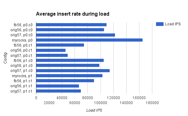
I only show the insert rate graph for SSD. The results with the disk array are similar. The insert rate is better for WiredTiger because it supports more concurrency internally courtesy of extremely impressive engineering. We have work in progress to make this much better for RocksDB.

Query performance

These display the query rates for 1, 4, 8, 16 and 24 concurrent clients using a disk array and then SSD. RocksDB does better than WiredTiger on both disk and SSD. RocksDB uses less random IO when writing changes back to storage and the benefit from this is larger with disk than with an SSD so the speedup for RocksDB is larger with the disk array.


Efficiency

This includes absolute and relative efficiency metrics from the tests run with 16 concurrent clients and SSD. The values are from vmstat and iostat run for the duration of the test. The absolute metrics are the per-second rates. The relative metrics are the per-second rates divided by the operation rate which measures HW consumed per insert or query. The operation rate is either the load rate (IPS) or the query rate (QPS).

The columns are:
  • cs.sec - average context switch rate
  • cpu.sec - average CPU load (system + user CPU time)
  • cs.op - context switch rate / operation rate
  • cpu.Kop - (CPU load / operation rate) X 1000
  • r.sec - average rate for iostat r/s
  • rkb.sec - average rate for iostat rKB/s
  • wkb.sec - average rate for iostat wKB/s
  • r.op - r.sec / operation rate
  • rkb.op - rkb.sec / operation rate
  • wkb.op - w.sec / operation rate


Load Efficiency

Conclusions from efficiency on the load step:
  • The context switch and CPU overheads are larger with RocksDB. This might be from mutex contention
  • I need more precision to show this but the relative write rate is much better for WiredTiger
  • The relative read rate is much better for WiredTiger. I suspect that some data is being read during compaction by RocksDB.

cs.sec  cpu.sec cs.op   cpu.Kop   r.sec   rkb.sec wkb.sec r.op    rkb.op  wkb.op  engine
182210  43      21.8    5.176     7.7     41      100149  0.001   0.005   0.000   RocksDB
108230  68      4.3     2.721     0.5     4       58327   0.000   0.000   0.000   WiredTiger

Query Efficiency

Conclusions from efficiency on the query step:
  • The CPU overheads are similar
  • The read and write overheads are larger for WiredTiger. RocksDB sustains more QPS because it does less IO for an IO-bound workload.

cs.sec  cpu.sec cs.op   cpu.Kop   r.sec   rkb.sec wkb.sec r.op    rkb.op  wkb.op  engine
87075   53      4.6     2.772     6394.2  52516   27295   0.338   2.774   1.442   RocksDB
65889   40      5.5     3.320     6309.8  88675   50559   0.529   7.437   4.240   WiredTiger

Results for disk

Results at 1, 4, 8, 16 and 24 concurrent clients for RocksDB and WiredTiger. IPS is the average insert rate during the load phase and QPS is the average query rate during the query phase.

clients IPS     QPS   RocksDB
1       3781    281
4       12397   1244
8       16717   1946
16      19116   2259
24      17627   2458

clients IPS     QPS   WiredTiger
1       5080    227
4       18369   726
8       35272   843
16      55341   808
24      64577   813

Results for SSD

Results at 1, 4, 8, 12, 16, 20 and 24 concurrent clients for RocksDB and WiredTiger. IPS is the average insert rate during the load phase and QPS is the average query rate during the query phase.

clients IPS     QPS   RocksDB
1       3772    945
4       12475   3171
8       16689   6023
12      18079   8075
16      18248   9632
20      18328   10440
24      17327   10500

clients IPS     QPS   WiredTiger
1       5077    843
4       18511   2627
8       35471   4374
12      43105   5435
16      55108   6067
20      62380   5928
24      64190   5762

Response time

This has per-operation response time metrics that are printed by Linkbench at the end of a test run. These are from the SSD test with 16 clients. While the throughput is about 1.5X better for RocksDB the p99 latencies tend to be 2X better with it. It isn't clear whether the stalls are from WiredTiger or storage.

For RocksDB:

ADD_NODE count = 893692  p50 = [0.2,0.3]ms  p99 = [3,4]ms  max = 262.96ms  mean = 0.37ms
UPDATE_NODE count = 2556755  p50 = [0.8,0.9]ms  p99 = [10,11]ms  max = 280.701ms  mean = 1.199ms
DELETE_NODE count = 351389  p50 = [0.8,0.9]ms  p99 = [11,12]ms  max = 242.851ms  mean = 1.303ms
GET_NODE count = 4484357  p50 = [0.5,0.6]ms  p99 = [9,10]ms  max = 262.863ms  mean = 0.798ms
ADD_LINK count = 3119609  p50 = [1,2]ms  p99 = [13,14]ms  max = 271.504ms  mean = 2.211ms
DELETE_LINK count = 1038625  p50 = [0.6,0.7]ms  p99 = [13,14]ms  max = 274.327ms  mean = 1.789ms
UPDATE_LINK count = 2779251  p50 = [1,2]ms  p99 = [13,14]ms  max = 265.854ms  mean = 2.354ms
COUNT_LINK count = 1696924  p50 = [0.3,0.4]ms  p99 = [3,4]ms  max = 262.514ms  mean = 0.455ms
MULTIGET_LINK count = 182741  p50 = [0.7,0.8]ms  p99 = [6,7]ms  max = 237.901ms  mean = 1.023ms
GET_LINKS_LIST count = 17592675  p50 = [0.8,0.9]ms  p99 = [11,12]ms  max = 26278.336ms  mean = 1.631ms
REQUEST PHASE COMPLETED. 34696018 requests done in 3601 seconds. Requests/second = 9632

For WiredTiger:

ADD_NODE count = 562034  p50 = [0.2,0.3]ms  p99 = [0.6,0.7]ms  max = 687.348ms  mean = 0.322ms
UPDATE_NODE count = 1609307  p50 = [1,2]ms  p99 = [20,21]ms  max = 1331.321ms  mean = 1.761ms
DELETE_NODE count = 222067  p50 = [1,2]ms  p99 = [20,21]ms  max = 1116.159ms  mean = 1.813ms
GET_NODE count = 2827037  p50 = [0.8,0.9]ms  p99 = [19,20]ms  max = 1119.06ms  mean = 1.51ms
ADD_LINK count = 1963502  p50 = [2,3]ms  p99 = [27,28]ms  max = 1176.684ms  mean = 3.324ms
DELETE_LINK count = 654387  p50 = [1,2]ms  p99 = [21,22]ms  max = 1292.405ms  mean = 2.761ms
UPDATE_LINK count = 1752325  p50 = [2,3]ms  p99 = [30,31]ms  max = 4783.055ms  mean = 3.623ms
COUNT_LINK count = 1068844  p50 = [0.3,0.4]ms  p99 = [4,5]ms  max = 1264.399ms  mean = 0.705ms
MULTIGET_LINK count = 114870  p50 = [1,2]ms  p99 = [17,18]ms  max = 466.058ms  mean = 1.717ms
GET_LINKS_LIST count = 11081761  p50 = [1,2]ms  p99 = [21,22]ms  max = 19840.669ms  mean = 2.624ms

REQUEST PHASE COMPLETED. 21856135 requests done in 3602 seconds. Requests/second = 6067 

Tuesday, November 24, 2015

Read, write & space amplification - B-Tree vs LSM

This post compares a B-Tree and LSM for read, write and space amplification. The comparison is done in theory and practice so expect some handwaving mixed with data from iostat and vmstat collected while running the Linkbench workload. For the LSM I consider leveled compaction rather than size-tiered compaction. For the B-Tree I consider a clustered index like InnoDB.

The comparison in practice provides values for read, write and space amplification on real workloads. The comparison in theory attempts to explain those values.

B-Tree vs LSM in theory


Read Amplification


Most comparisons should be done for a specific context including the hardware and workload. For now I am only specific about the cache hit rate. For the B-Tree I assume that all non-leaf levels are in cache. For the LSM I assume that everything but the data blocks of the largest LSM level are in cache. While an LSM with leveled compaction has more things to keep in the cache (bloom filters) it also benefits from a better compression rate and the cache requirements are similar to a clustered B-Tree.

Worst-case disk read-amp for point queries is 1 for the B-Tree and the LSM as one block is read from the B-Tree leaf level and largest LSM level. Disk read-amp for range queries is 1 or 2 for a short range scan assuming that 1 or 2 blocks from the B-Tree leaf level and LSM max level are read. Note the impact of my assumption for cached data. While many files might be accessed for a short range query with an LSM everything but the max level data blocks are in cache.

The number of key comparisons can be used as the in-memory read-amp. For a B-Tree with 1M keys there are about 20 key comparisons on a point query. For a range query with a B-Tree there is one additional comparison for each row fetched.

It is harder to reason about the number of comparisons for an LSM. Bloom filters can be used for a point query to avoid comparisons but when there are too many files in level 0 then there will be too many bloom filter checks. Bloom filters don't work for range queries, ignoring prefix bloom filters. When query processing is IO-bound I don't expect key comparison overhead to make a difference between an LSM and B-Tree. So I will ignore this for now.

If you want to maximize the ratio of the database to cache sizes while doing at most one disk read per point query then an LSM with leveled compaction or a clustered B-Tree are the best choices. For a clustered B-Tree the things that must be in memory are one key per leaf block and all non-leaf levels of the index. An LSM with leveled compaction has similar requirements, although it also needs some of the bloom filters to be in memory.

The cache requirement is much larger for an LSM with size-tiered compaction. First, the max level has ~50% of the data compared to ~90% with leveled compaction and it less likely that all data except the max file are in cache. Second, there are more old versions of key-value pairs, space-amp is larger, so there is more data that needs to be in the cache.

An unclustered B-Tree index also requires more memory to keep the important bits in cache. The important bits are all keys, which is much more memory than one key per leaf block for a clustered B-Tree.

Write Amplification


For now I assume that flash storage is used so I can focus on bytes written and ignore disk seeks when explaining write-amp. For a B-Tree a change is first recorded in the redo log and the page is eventually written back. The worst case occurs when the buffer pool is full with dirty pages and reading the to-be-modified page into the buffer pool forces a dirty page to be evicted and written back. In this case there is a redo log write and a page write back per row change. If the row is 128 bytes and the page is 4096 bytes then 4096+128 bytes are written to storage per 128 byte row change. The write-amp is 33 -- (4096 + 128) / 128. The write-amp is reduced when there is more one changed row on a page or when one row is changed many times before write back.

For the LSM the redo log is written immediately on a row change. When the memtable is full and flushed to level 0 then the row is written again. When level N is full and compaction is done from level N to level N+1 then one SST file is read from level N, ~10 SST files are ready from level N+1 and ~10 files are written back to level N+1. The write-amp to move rows from level N to N+1 is ~10 given my handwaving but in practice it is ~7 and I am waiting for a paper to be published to explain that. The total write-amp is computed from the writes required to move a row change from the memtable to the max level. The write-amp is 1 for the redo log, 1 for the memtable flush and usually ~1 for compacting to level 1. Assuming the LSM has levels 0 to 4 and the per-level write-amp is 7 for levels 2 to 4 then the total write-amp is 24 -- 1 + 1 + 1 + 7 + 7 + 7.

From the examples above the LSM has less write-amp than the B-Tree but those examples were not meant to be compared. An LSM tends to have less write-amp than a B-Tree. When using flash storage this means the device will last longer. When using disk storage this is likely to save more IO capacity for reads leading to higher QPS.

The IO pattern for a busy LSM is concurrent streams of IO. Each stream writes files sequentially, but the writes from different streams can end up in the same logical erase block (logical means it is striped across many NAND chips). The level of the leveled compaction LSM predicts the lifetime of the write. Writes to level 0 have a short lifetime. Writes to level 4 have a much longer lifetime. The write rates per level are similar -- there might be 10 MB/second of writes to levels 0 and 1 and then 20 MB/second of writes to levels 2 through 4. This means that logical erase blocks will end up with a mix of long and short lived data and the long-lived data will get copied out during flash garbage collection. Does your flash device use logical erase blocks? If it does then there will be write-amp from flash GC even with an LSM. Flash devices that support multi-stream will help a lot.

Space Amplification


A B-Tree gets space-amp from fragmentation, per-row metadata and fixed page sizes on disk. The leaf pages in a B-Tree are between 50% and 70% full when subject to random updates. When they are 2/3 full then space-amp is 1.5 and when they are 1/2 full then space-amp is 2. An update-in-place B-Tree like InnoDB uses ~20 bytes/row for metadata to support consistent read and transactions. The metadata overhead is much smaller for an LSM like MyRocks. Finally, when compression is done for InnoDB there will be wasted space because page sizes are fixed on disk. When a 16kb in-memory page compressed to 5kb for a table that uses 8kb pages on disk, then 3kb of the 8kb page on disk is wasted.

An LSM gets space-amp from old versions of key-value pairs. Leveled and size-tiered compaction differ significantly in this regard. With leveled compaction you are likely to get space-amp of 1.1 or 1.2 and with size-tiered compaction a more common result is space-amp of 2. Size-tiered compaction can suffer even more from additional but temporary space-amp when the max file is compacted and disk space is required for the old and new version of that file.

Compression reduces space-amp and for this reason I claim that space-amp of less than 1 is possible.


B-Tree vs LSM in practice


This post is longer than I expected, so I will write less here. This is a good spot for a joke about space-amp and write-amp. I have begun reporting on read, write and space amplification by normalizing the server's IO and CPU rates by QPS during benchmarks. I use iostat to get data for on-disk read-amp and write-amp by measuring reads/second, MB read/second and MB written/second. I frequently ignore writes/second because that mixes fast and slow writes (redo log writes are fast, page writes are slow). I use vmstat to measure the CPU utilization and that is a proxy for the in-memory read-amp and write-amp. Finally I look at the size of the database on disk to compare space-amp. The data is usually measured over 1 hour intervals to make it easy to detect when metrics get worse as a database ages. I try to run workloads for at least 12 hours to give things time to go bad.

Percona has begun doing this for some benchmark reports. I hope this becomes a common practice.

This is an example from running Linkbench for MongoDB with RocksDB and WiredTiger. I will soon have more results for MyRocks. I am thrilled that we have a copy-on-write B-Tree (WiredTiger) and an LSM (RocksDB) available as storage engines in MongoDB. We are also bringing RocksDB to MySQL via the MyRocks effort. The big deal for MyRocks compared to InnoDB is half the space-amp and half the write-amp. This has been measured on Linkbench and on the real workload. This is a big deal.

Monday, November 23, 2015

Read, write & space amplification - pick 2

Good things come in threes, then reality bites and you must choose at most two. This choice is well known in distributed systems with CAPPACELC and FIT. There is a similar choice for database engines. An algorithm can optimize for at most two from readwrite and space amplification. These are metrics for efficiency and performance. This means one algorithm is unlikely to be better than another at all three. For example a B-Tree has less read amplification than an LSM while an LSM has less write amplification than a B-Tree. I abbreviate the metrics as read-amp, write-amp and space-amp. I also abbreviate this as the framework.

The framework assumes a database workload that consists of point-queries, range-queries of length N and writes. Were I to add a delete operation then this would match the RocksDB and LevelDB API. The write is a blind-write as it doesn't imply a read prior to the write.

This is part one of a topic that requires several blog posts. The second post will compare a B-Tree and LSM using the framework. The third post will argue that an algorithm cannot be optimal for all three metrics.

Purpose


Read, write and space amplification explain performance and efficiency when evaluating algorithms for real and potential workloads. They aren't a replacement for Big O notation. They usually assume a specific workload and configuration including RAM size, database size and type of storage.

We began using the framework to compare InnoDB and RocksDB because better performance is an insufficient metric on which to choose an algorithm. Endurance (write amp) and capacity (space amp) matter when using flash. IOPs (read amp for point and range queries, write amp for writes) matters when using disk.

The framework is useful for understanding the compromises made in search of better QPS. It is easy to trade write for space or read efficiency in write-optimized algorithms but these trades should be disclosed because they are not free. New algorithms can show better write throughput than RocksDB by making range reads less efficient but the Linkbench workload needs efficient writes and efficient range reads.

The framework is useful because key comparisons aren't created equal. Traditional algorithm analysis is great for understanding in-memory performance via bounds on the number of key comparisons. But big-O notation is harder to use when some keys are read from cache, others from RAM and some from disk. Constant factors matter. The difference between 1.2 and 1.5 disk reads per query can be a big deal.


Read amplification


Read-amp is the amount of work done per logical read operation. This can be defined for in-memory databases, persistent databases assuming no cache (worst-case behavior) and persistent databases assuming some cache (average-case behavior). The work done in-memory can be the number of key comparisons and traditional algorithm analysis can be used. The work done on-disk includes the number of bytes transferred and seeks (seeks matter on disks, not on NVM). The work done can also include the cost of decompressing data read from storage which is a function of the read block size and compression algorithm.

Read-amp is defined separately for point and range queries. For range queries the range length matters (the number of rows to be fetched). In Linkbench the average range query fetches about 20 rows.

Read-amp can also be defined for point queries on keys that don't exist. Some algorithms use a bloom filter to avoid disk IO for keys that don't exist. Queries for non-existent keys is common in some workloads. Bloom filters can't be used for a range query. The most frequent query in Linkbench is a range query that includes an equality predicate on the first two columns of the range query index. With RocksDB we define a prefix bloom filter to benefit from that.


Write amplification


Write-amp is the amount of work done per write operation. This can include the number of bytes written to storage and disk seeks per logical write operation. This can be split into in-memory and on-disk write-amp but I frequently ignore in-memory write-amp.

There is usually a cost to pay in storage reads and writes following a logical write. With write-amp we are ignoring the read cost. The read cost is immediate for an update-in-place algorithm like a B-Tree as a page must be read to modify it. The read cost is deferred for a write-optimized algorithm like an LSM as compaction is done in the background and decoupled from the logical write. There is usually some write cost that is not deferred - updating in-memory structures and writing a redo log.

With flash storage there is usually additional write-amp from the garbage collection done by the FTL to provide flash blocks that can be rewritten. Be careful about assuming too much about the benefit of sequential and large writes from a write-optimized database engine. While the physical erase block size on a NAND chip is not huge, many storage devices have something that spans physical erase blocks when doing GC that I will call a logical erase block. When data with different lifetimes ends up in the same logical erase block then the long-lived data will be copied out and increase flash GC write-amp (WAF greater than 1).  I look forward to the arrival of multi-stream to reduce flash GC WAF.

Space amplification


Space-amp is the ratio of the size of the database to the size of the data in the database. Compression decreases space-amp. It is increased by fragmentation with a B-Tree and old versions of rows with an LSM. A low value for space-amp is more important with flash storage than disk because of the price per GB for storage capacity.

Efficiency & Performance


I work on small data systems. Small data is another name for OLTP. Small data workloads are highly concurrent and with concurrency better efficiency usually implies better performance. But performance and efficiency are not always strongly correlated. For example an algorithm with a high read-amp for range queries might hide the extra latency by doing disk reads in parallel. This improves response time but doesn't improve efficiency and the algorithm with less read-amp will sustain more QPS at higher concurrency.

Wednesday, November 18, 2015

How does MongoDB do on Linkbench with concurrency?

I started to study performance math with a focus on queueing theory and the USL. To get data for the USL I ran Linkbench for MongoDB with different levels of concurrency. I tested WiredTiger in MongoDB 3.2.0rc0 and 3.0.7 and then RocksDB in MongoDB 3.2.0. The performance summary is:
  • WiredTiger load scales much better in 3.2 compared to 3.0
  • RocksDB throughput is stable at high concurrency
  • WiredTiger 3.2 throughput is stable at high concurrency. For WiredTiger 3.0 the load rate drops significantly at high concurrency and the query rate also has an odd drop.

Configuration


The test server has 2 sockets with 6 CPU cores/socket and hyperthreading enabled to get 24 HW threads. The server also has 6 SAS disks with HW RAID 0 and 1 SSD. I intended to use the disk array for all tests but ended up using the SSD for the WiredTiger 3.0.7 test. The server also has 144G of RAM and the test database was cached by mongod for all tests. The oplog was enabled but sync-on-commit was not done. For Linkbench I set maxid1 to 10M and the test pattern was load, run for 30 minutes, run for 30 minutes and the query rate is reported for the second 30 minute run. Snappy compression was used for all tests. The test was run for 1 to 48 concurrent clients with MongoDB 3.2.0 and stopped at 30 concurrent clients for MongoDB 3.0.

Data


Results are on gist.github for the load and query tests.

Load

WiredTiger  throughput for write-heavy workloads is much better in 3.2 than 3.0 as I previously reportedFrom PMP output it looks like WiredTiger in MongoDB 3.0 suffers from too frequent plan-cache invalidation that I wrote about this previously. I think RocksDB insert performance saturates earlier from mutex contention on the memtable writer mutex. 

Query


WiredTiger performance is the same for 3.0 and 3.2 until 21 concurrent clients. At that point the performance for 3.0 drops and response time for all operations is slower (reads & writes). This is odd and I won't try to debug it. For RocksDB I have an educated guess at the problem (need to use SingleDelete optimization in MongoRocks to reduce overhead from tombstones) to explain why throughput for it is worse than WiredTiger.


Thursday, November 12, 2015

Define better for a small-data DBMS

There are many dimensions by which a DBMS can be better for small data workloads: performance, efficiency, manageability, usability and availability. By small data I mean OLTP. Performance gets too much attention from both industry and academia while the other dimensions are at least as important in the success of a product. Note that this discussion is about which DBMS is likely to get the majority of new workloads. The decision to migrate a solved problem is much more complex.

  • Performance - makes marketing happy
  • Efficiency - makes management happy
  • Manageability - makes operations happy
  • Usability - makes databased-backed application developers happy
  • Availability - makes users happy

Performance makes marketing happy because they can publish a whitepaper to show their product is faster than the competition and hope that the message morphs from X is faster than Y in this context into X is faster than Y. This is the art of benchmarketing. It can be risky to use average throughput as a performance metric unless there was a response time SLO. Otherwise good average throughput can hide lousy variance like the page writeback stalls in InnoDB that Percona spent a lot of time making better. When a benchmark result doesn't include an SLO then you need to see throughput over time or response time histograms (response time at the 95th percentile for example).

Efficiency makes management happy because less hardware is able to do more work. A simple way to report this is to list the amount of disk IO and CPU used per transaction by dividing rates from iostat and vmstat by the QPS or TPS as I have been doing in recent benchmark reports. Better efficiency might not imply better response time but it usually implies better throughput for highly concurrent workloads. Efficiency has several dimensions including read, space and write and one database engine is unlikely to be optimal for all of them, but that is for another blog post.

Manageability makes life easier for the operations team that supports the DBMS. They shouldn't waste time manually fixing problems when the fix can be automated. Oncall week shouldn't mean you wake up every few hours to replace failed servers. Replacement of failed masters for MySQL isn't automated at many web-scale MySQL deployments and I feel sorry for the oncall at those places. With MySQL 5.7 the pieces exist for a solution and I hope these are combined into an open-source solution similar to what we have

Usability makes life easier developers who write database-backed applications. Developers shouldn't spend time reinventing the wheel, thus my expectation of per-shard support for consistent read and transactions. A declarative query language and good-enough query optimizer also make life easier for everyone. I consider the MongoDB query API to be declarative. My feature list is longer but I won't include it here.

Availability - this makes users happy. There is big and small downtime. Both can significantly reduce availability. An example of big downtime is taking 30 minutes to replace a failed master. An example of small downtime is slow commit courtesy of synchronous geo-replication. Small downtime doesn't get enough attention. When commit to one row takes 100 milliseconds and the workload demands 100 commits/second to that row then there will be 90 commits/second that can't get done and the user experience for can't get done is similar to database down.

MySQL and MongoDB


It is interesting to compare the upcoming releases of MongoDB (3.2) and MySQL (5.7) by these metrics. MongoDB has a large lead in manageability for web-scale deployments (sharded replica sets) and this continues with the 3.2 release. MongoDB comes with support for failover automation, while MySQL does not. MongoDB 3.2 has the potential to provide much better availability than a MySQL deployment that lacks automated master failover (we have that, upstream MySQL does not) although the new code in MongoDB needs time to mature.

MySQL has a large lead in performance based on the benchmarks I have run. Better response time and throughput are important but won't determine whether MongoDB or MySQL is chosen for a new workload. MySQL also has a large lead in usability because many workloads need per-shard transactions, per-shard consistent read and per-shard joins. It isn't hard to add support for per-shard transactions and consistent read to MongoDB given they are already provided by WiredTiger and RocksDB and I expect the MongoDB to match MySQL in usability in the next few years.

MongoDB and MySQL are similar for efficiency. Both have read & write optimized engines including MongoRocks and MyRocks for write optimized.

How does this end? MongoDB becomes better by improving usability. MySQL becomes better by improving manageability and availability. Both have long track records of steady improvement although MongoDB is moving faster. The product that gets there first is likely to get the majority of new workloads.

Wednesday, November 4, 2015

MongoDB 3.2 vs Linkbench

I used LinkbenchX to compare performance and efficiency for MongoDB 3.2.0rc0 vs 3.0.7 with the RocksDB and WiredTiger engines. The Linkbench test has two phases: load and query. The test was run in three configurations: cached with data on disk, too big to cache with data on disk and too big to cache with data on SSD. My summary:

Performance:
  • load rates are similar for disk and SSD with RocksDB and WiredTiger
  • load rate for WiredTiger is ~2X better in 3.2 versus 3.0
  • load rate for WiredTiger is more than 2X better than RocksDB
  • query rate for WiredTiger is ~1.3X better than RocksDB for cached database
  • query rate for RocksDB is ~1.5X better than WiredTiger for not cached database
Efficiency:
  • disk space used is ~1.33X higher for WiredTiger vs RocksDB
  • disk bytes written per document during the load is ~5X higher for RocksDB
  • disk bytes written per query is ~3.5X higher for WiredTiger
  • RocksDB uses ~1.8X more CPU during the load
  • WiredTiger uses ~1.4X more CPU during the query phase
  • with a 32G block cache mongod RSS is ~42G with WiredTiger vs ~34G with RocksDB

LinkbenchX


LinkbenchX is a fork of Linkbench. Source for Linkbench and LinkbenchX is in github. LinkbenchX adds support for MongoDB and an option to sustain a fixed request arrival rate. For this test I use the MongoDB support but not the fixed request arrival rate by using bin/linkbench from Linkbench. I am grateful to Percona for porting Linkbench to MongoDB.

The Linkbench workload requires transactions to update the count collection when a document is added to or removed from the link collection. MongoDB doesn't support per-shard transactions and the Linkbench results will be incorrect. I understand that cross-shard transactions are hard, but per-shard transactions and per-shard consistent read are valuable for Linkbench and for selling to the enterprise. I hope they arrive in MongoDB 3.4.

Linkbench is run in two phases: load and query. I configured Linkbench to use 12 threads for both phases. The query phase was done as a sequence of 1-hour tests to measure whether performance and efficiency changed over time.

For the cached database test I set the value of maxid1 in the Linkbench file config/FBWorkload.properties to 50,000,001 and the database block cache to 32G. The database was cached by the OS but not WiredTiger or RocksDB in this setup as the compressed database was ~50G.

For the not cached database test I set the value of maxid1 to 250,000,001, the database block cache to 8G and started a background process to use mlock to leave at most 40G for mongod and the OS page cache. The database was at least 150G and the workload used lot of storage IO.

For all tests I changed the Linkbench file config/LinkConfigMongoDBv2.properties to use transaction_support_level=1, requesters=12, loaders=12, maxtime=3600, requestrate=0 and requests=100000000000. Fsync is not done on commit.

The test server has 24 cores with hyperthreading enabled, 144G of RAM and either one 400G SSD (Intel DC s3700) or 6 SAS disks with HW RAID 0. The server uses Fedora release 19, Linux 3.14.27-100, gcc 4.8.3 and MongoDB was linked with tcmalloc.

Snappy compression was used for both RocksDB and WiredTiger. For all tests this was in the mongod configuration file:
processManagement:
  fork: true
systemLog:
  destination: file
  logAppend: true
storage:
  syncPeriodSecs: 600
  journal:
    enabled: true
storage.wiredTiger.collectionConfig.blockCompressor: snappy
storage.wiredTiger.engineConfig.journalCompressor: none
For the not cached database this was in the mongod configuration file:
replication.oplogSizeMB: 4000
storage.wiredTiger.engineConfig.cacheSizeGB: 8
storage.rocksdb.cacheSizeGB: 8
For the cached database this was in the mongod configuration file:
replication.oplogSizeMB: 8000
storage.wiredTiger.engineConfig.cacheSizeGB: 32
storage.rocksdb.cacheSizeGB: 32

Legend

The legend for the data in the following sections. The disk and CPU metrics are collected from iostat and vmstat. Most rates below are normalized by the rate for operations/second where operation is an insert during the load phase and query during the query phase. The real insert rate across all collections is reported for ops below but I use the number of inserts to the node collection (50M or 250M) when normalizing the iostat and vmstat rates.

  • ops - average rate for operations/second (inserts or queries per second)
  • db.gb - database size in GB (two numbers are from du without and with --apparent-size)
  • r/o - disk reads per operation
  • wKB/o - disk KB written per operation
  • cs/o - context switches per operation
  • cpu/o - CPU/operation from vmstat us+sy divided by ops multiplied by 1M 
  • rss - RSS from ps for the mongod process
  • setup - wt (wiredtiger), rx (rocksdb), 307 (mongo 3.0.7), 320 (mongo 3.2.0rc0), op0/op1 - oplog off/on

Cached database

For this test there were 50M, ~220M and X docs in the node, link and count collections after the load phase. In addition to the conclusions listed at the top of this post, WiredTiger 3.2 vs 3.0 uses less CPU and has fewer context switches per insert. It is good to see it become more efficient and the insert rate for WiredTiger has almost doubled from 3.0 to 3.2. 

The context switch rate per insert is much larger for RocksDB because of the global mutex that serializes inserts into the memtable. There are no disk reads during this test because the database fits in the OS page cache. The CPU rate for WiredTiger is also much higher during the load. That might be a side effect of more mutex contention.

The difference in database sizes for WiredTiger vs RocksDB is small after the load but grows quickly during the run phases. I did not try to debug it but the growth for WiredTiger could be a problem. WiredTiger also uses much more memory than RocksDB. But I don't know whether that is a fixed overhead (~8G) or a relative overhead (30% of the block cache size).

Using the oplog doubles the wKB/o rate because writes are done twice -- once to the oplog, once to the database. The internal write-amplification reported by RocksDB for rx.320.op1 is 6.1.

--- load
ops    db.gb   r/o     wKB/o   cs/o    cpu/o   setup
51416  53/36   0.0     1.355    2.8    2171    wt.320.op0
46156  44/40   0.0     2.316    4.0    2460    wt.320.op1
28171  47/41   0.0     1.358    0.9    3161    wt.307.op0
28080  46/35   0.0     2.304    1.8    3520    wt.307.op1
26654  31/31   0.0     5.318   16.0    3787    rx.320.op0
19033  36/36   0.0     11.643  18.4    4881    rx.320.op1

--- run, 2nd hour
ops     db.gb   r/o    wKB/o   cs/o    cpu/o   rss   setup
14483   86/72   0.0    2.486    3.6    2170    42G   wt.320.op1
14312   78/71   0.0    2.338    3.6    2259    43G   wt.307.op1
10794   38/38   0.0    1.357    3.9    2470    35G   rx.320.op1

--- run, 12th hour
ops     db.gb   r/o    wKB/o   cs/o    cpu/o   rss   setup
13042   100/90  0.0    2.588    4.1    2378    36G   wt.320.op1
12742   94/88   0.0    2.623    4.0    2414    43G   wt.307.op1
10550   45/45   0.0    1.491    4.1    2533    35G   rx.320.op1

Not cached, disk array

For this test there were 250M, 1B and X documents in the node, link and count collections after the load phase. The database did not fit in RAM and the disk array can do ~1200 IOPs. The query phase was run for 24 hours.

The new result here is that RocksDB sustained a much higher QPS rate during the query phase. From the response times listed at the end of this post the difference appears to be a better response time for the most frequent operation -- GET_LINKS_LIST -- which is a short range scan. RocksDB also benefits from a better cache hit rate because the database is smaller and the r/o rate is slightly smaller. It also uses less IO capacity for writes (wKB/o is smaller and writes are less random) leaving more IO capacity for reads.

-- load
ops    db.gb    r/o     wKB/o   cs/o    cpu/o   setup
40667  191/177  0.0     2.319    2.8    2803    wt.320.op1
25149  191/178  0.0     2.306    1.8    4041    wt.307.op1
18725  153/153  0.0    11.568   18.7    4968    rx.320.op1

--- run, 2nd hour
ops    db.gb    r/o     wKB/o   cs/o    cpu/o   rss   setup
504    199/188  0.842   5.326    8.0    5481    12G   wt.320.op1
507    206/187  0.798   5.171    7.5    8013    13G   wt.307.op1
850    153/153  0.746   1.743    5.3    3684    11G   rx.320.op1

--- run, 12th hour
ops    db.gb    r/o     wKB/o   cs/o    cpu/o   rss   setup
491    196/195  0.831   5.173    8.1    5700    12G   wt.320.op1
488    195/195  0.794   5.273    7.6    8380    12G   wt.307.op1
864    155/155  0.725   1.588    5.4    3967    11G   rx.320.op1

--- run, 24th hour
ops    db.gb    r/o     wKB/o   cs/o    cpu/o   rss   setup
494    199/197  0.799   5.404    8.1    5615    10G   wt.320.op1
471    197/197  0.814   5.303    7.8    8564    12G   wt.307.op1
833    156/156  0.738   1.721    5.5    4301    10G   rx.320.op1

Not cached, SSD

RocksDB sustained a higher QPS than WiredTiger for the query phase similar to the result for a disk array with a not cached database. I didn't expect that result here or for the disk array.

--- load
ops    db.gb    r/o     wKB/o   cs/o    cpu/o   setup
40742  195/180  0.0     2.318    2.9    2798    wt.320.op1
25308  188/177  0.0     2.306    1.8    4007    wt.307.op1
18603  155/154  0.0    11.458   18.6    5005    rx.320.op1

--- run, 2nd hour
ops    db.gb    r/o     wKB/o   cs/o    cpu/o   rss   setup
3870   229/213  0.821   4.869   6.3     4179    11G   wt.320.op1
3814   228/210  0.813   4.620   6.1     4163    13G   wt.307.op1
6146   155/155  0.735   1.344   5.3     3063    11G   rx.320.op1

--- run, 12th hour
ops    db.gb    r/o     wKB/o   cs/o    cpu/o   rss   setup
3715   232/221  0.855   4.810   6.6     4449    9G    wt.320.op1
3415   223/217  0.825   4.582   6.4     4332    11G   wt.307.op1
5827   162/162  0.776   1.356   5.6     3239    11G   rx.320.op1

Response time metrics

These are response time metrics for each configuration. These are printed by Linkbench at the end of each run. The most interesting result is for the GET_LINKS_LIST operation which uses a short range scan (~10 rows on average). For the cached database, the p99 for RocksDB is ~14ms vs ~3ms for WiredTiger. I think the problem for RocksDB is from too many tombstones. We recently came up with a more efficient way to remove them in MyRocks. The p99 for RocksDB in the not cached databases (disk & SSD) is better than WiredTiger and ~12ms for ssd, ~47ms for disk. 

RocksDB compaction stats

This is the compaction IO statistics from RocksDB at the end of the 24th 1-hour query run for the no cached, disk configuration.

Sunday, October 11, 2015

Losing it?

Many years ago the MySQL team at Google implemented semi-sync replication courtesy of Wei Li. The use case for it was limited and the community was disappointed that it did not provide the semantics they wanted. Eventually group commit was implemented for binlog+InnoDB: first by the MySQL team at Facebook, then much better by MariaDB, and finally in upstream MySQL. With group commit some magic was added to give us lossless semisync and now we have automated, lossless and fast failover in MySQL without using extra replicas. This feature is a big deal. I look forward to solutions for MariaDB (via binlog server and MaxScale) and MySQL (via Fabric and Proxy).

MongoDB is ahead of MySQL in features that make scale-out easier to manage and the next release (3.2) adds a few more features and more robust code for existing features. I hope that some of the features that have been sacrificed in the name of scale-out will eventually arrive in a MongoDB release: per-shard transactions, per-shard joins, per-shard consistent read.

Behavior


Many times we describe algorithms when users need to understand behavior and then the user gets lost in the details. It is important for developers to understand when transactions can be lost and I will describe that with answers to two questions.
  1. After the changes from a commit are visible to a concurrent session under what conditions can that commit be lost?
  2. After a client has been informed that a commit has succeeded under what conditions can that commit be lost?


Details


I list four combinations of behavior to consider and the features in MySQL and MongoDB that provide them:


Editorial


MySQL uses one solution (lossless semisync) to protect against both loss of visible and acknowledged commits. With lossless semisync row locks are held on the master until at least one slave acknowledges the commit. This can reduce commit throughput as there is a network round trip between master and replica(s) before commit is finished and row locks are released. There is at one network round trip between commits to the same row. This overhead is reduced by moving the replica close to the master. In the solution described by Yoshinori the binlog archive provides the ack rather than using extra replicas in every data center and because the binlog archive doesn't require a lot of hardware it is easier to move it closer to the master.

In MongoDB total protection comes from two solutions -- majority read concern and write concern. The benefit is that majority write concern doesn't make commit slower assuming a workload has sufficient concurrency. It will add latency to each client doing a commit just like MySQL semisync. A different feature, majority read concern, protects against loss of a visible commit. However, there is the risk that a client that needs read-your-own write semantics will have to wait. At this point it isn't clear to me that MongoDB makes it easy to read your own writes. I wonder if applications that care more about performance will use majority read concern without using majority write concern. That isn't an option with MySQL.

It will take time to figure out the implications of the performance differences. With MySQL delays are added to writers as it takes them longer to get the through semi-sync commit protocol. With MongoDB delays might be added to readers as they wait for the majority read snapshot to be advanced.


Durable on a slave?


It can be important to understand how durable a change is on a replica when the replica acknowledges a transaction to the master. There are several options and I have not read enough recent MySQL or MongoDB documentation to determine whether there are options beyond durable in memory:
  1. durable in memory - the commit is buffered in memory on a replica before it acks. Many years ago when we implemented semi-sync for MySQL this was the only choice. I tend to think that durable in memory is an oxymoron, but I am a pessimist.
  2. durable in a log - the commit is durable in a log file on a replica before it acks. There has been talk that MySQL would 
  3. committed on the replica - the commit is applied on a replica before it acks. That guarantees read-your-writes semantics when that replica is queried soon after committing a change on a master. Alas this is also likely to create performance lag unless the replica uses many threads to apply changes concurrently, just like on the master. It also creates a window where a commit is visible on a replica before the master.

More editorial


MongoDB documentation has tended to be optimistic about the features provided by the software. I think this will be resolved as the community grows. There have been some interesting discoveries. Hopefully the gap between documented and actual behavior will be reduced over time.

The mmap engine releases the per-database or per-instance write lock before syncing the oplog even when durable writes are requested.  This is now described as read uncommitted, but read non-durable might be a better name because reads are still consistent but you can see changes from others before those changes are durable in the oplog. I wrote about this when reading code and the docs have been updated since then but I think their docs need more edits. This is only a problem for the mmap engine and multiple engines in MongoDB means they need to be clear about behavior for mmap versus WiredTiger.

There were too strong claims about the semantics of the majority write concern. It protects against the loss of an acknowledged commit but some docs suggested it protected against the loss of a visible commit. Aphyr, an expert in distributed systems testing, highlighted this problem in his Call Me Maybe series and a bug report. I wrote about part of the problem prior to that but I did not connect the problem with the too-strong claims in the documentation. Many years ago MySQL made a similar mistake when documenting semi-sync replication and fixed their docs after I filed a bug.

Documentation claimed that 2-phase commit was used to keep config servers in sync. That makes it more likely that commit is all-or-nothing for the 3 or 5 config servers hosting the same data. Alas it can lead to read-only mode when a server goes away. I read the code and the two phases were 1) ping all config servers and then if all responded 2) send the change to all config servers. If all servers did not respond with OK then manual intervention was required. This isn't 2 phase commit. Fortunately, something much better will be done for the 3.2 release and the docs have been updated.

Finally, read the excellent series of posts from Tokutek on replica set failover including the overview and posts one, two, three and four. There have been problems that haven't been widely known. Fortunately the 3.2 release of MongoDB should make things better.

Wednesday, October 7, 2015

Problems not worth fixing

I worked on a closed-source DBMS years ago and the development cycle was 1) code for 6 months 2) debug for 18 months. Part 2 was longer than part 1 because the customers have high expectations for quality and the product delivers on that. But it was also longer because some co-workers might not have been code complete after 6 months and were quietly extending part 1 into part 2.

I fixed many bugs during part 2. One that I remember was in the optimizer. Someone added code to detect and remove duplicate expressions (A and A and B --> A and B). Alas the algorithm was O(N*N). Analytics queries can have complex WHERE clauses and all queries were forced to pay the O(N*N) cost whether or not they had any duplicate expressions. 

The overhead for this feature was reasonable after I fixed the code but it raises an interesting question. Are some problems not worth the cost of prevention? Several times a year I see feature requests that make me think of this.

Forgot to add the bug that inspired this post. In bug 30342 there was a change in the MySQL 5.0 optimizer that added predicates which could increase the overhead for query optimization when more predicates means more calls to records_in_range.

Monday, October 5, 2015

MyRocks versus allocators: glibc, tcmalloc, jemalloc

I used a host with Fedora 19 and Linkbench to determine the ability of memory allocators to avoid fragmentation with MyRocks (MySQL+RocksDB). RocksDB can create pressure on an allocator because allocations for the block cache can have a short lifetime. Memory is allocated on page read and released when a page is evicted from the cache. The allocation is the size of the decompressed page and sometimes the size of the compressed page. RocksDB puts more pressure on the allocator than InnoDB because with InnoDB the buffer pool allocation is done once at process start. After the Linkbench load finished I ran the query test for 24 hours and report the values of VSZ and RSS from ps at the end. From the results below jemalloc & tcmalloc do much better at avoiding fragmentation (value of RSS) compared to glibc 2.1.7. I am still adjusting to larger values of VSZ with jemalloc. It isn't a problem, but it takes time to accept.

VSZ       RSS       allocator
22246784  10062100  jemalloc
13600032  10545284  tcmalloc
26136152  20313268  glibc

Test details:
  • Linkbench with maxid=100M, loaders=10, requesters=20
  • MyRocks with 8G block cache for RocksDB
  • libc is glibc 2.17, tcmalloc from gperftools 2.1, jemalloc 3.6.0

Friday, October 2, 2015

Wanted: a file system on which InnoDB transparent page compression works

I work on MyRocks, which is a MySQL storage engine with RocksDB. This is an alternative to InnoDB. It might be good news for MyRocks if transparent page compression is the future of InnoDB compression. I got more feedback from the MySQL team that despite the problems I have reported, transparent page compression works. I was just testing the wrong systems.

So I asked core developers from Btrfs whether it was OK to do punch hole per write and they politely told me to go away. Bcachefs might be a great way to add online compression to a b-tree without doing punch hole per write but it is not ready for production. Someone from MySQL suggested I try ext4 so I setup two servers with Ubuntu 14.04 which is on the list of supported systems. I used XFS on one and ext4 on the other.

XFS was still a problem and ext4 was just as bad. The problem is that the unlink() system call takes a ridiculous amount of time after a multi-GB file has been subject to many punch hole writes. By ridiculous I mean 50X or 100X longer. Maybe I am the only one using InnoDB file-per-table and measuring time to drop a table or database. Bad things happen when DROP takes 10+ minutes --InnoDB is unusable by other connections and an InnoDB background thread might kill mysqld because it thinks there is an internal deadlock.

Did I mention this was good news for MyRocks? If you want compression then we get 2X better compression compared to compressed InnoDB. We also made sure that DROP TABLE and DROP INDEX are fast.

I updated bug 78277 for this problem. I am the only person updating that bug. I also found a corruption bug with transparent page compression, bug 78672. Past experience with transparent page compression is described here, here and here.

The end to my testing day was perfect. I rebooted the host to get back memory from XFS metadata allocations and the filesystem came back corrupt. Being a pessimist I was using a scratch filesystem for this, so I didn't lose my Ubuntu install.

Tuesday, September 8, 2015

Third day with InnoDB transparent page compression

My first two days with InnoDB transparent page compression didn't turn out well. Transparent page compression can make InnoDB source code simpler and InnoDB more performant on insert heavy workloads. Unfortunately the versions of XFS that I use are not happy after doing a hole-punch on write. The performance summary is that with transparent compression:

  • Database load is slightly faster
  • Transaction processing is slightly slower
  • DROP TABLE is 43X slower

MySQL 5.6 vs 5.7

I used a host with 24 HW threads, 144G of RAM and a 400G Intel s3700 SSD. The server uses Fedora 19, XFS and Linux kernel 3.14.27-100.fc19. The benchmark application is linkbench and was run with maxid1=100M, loaders=10 and requesters=20 (10 clients for the load, 20 for queries). I compared the Facebook patch for MySQL 5.6 with upstream MySQL 5.7. For 5.6 I used old-style compression for linktable and counttable. For 5.7 I used transparent compression for all tables. I also used 32 partitions for 5.6 and no partitions for 5.7. After the database was loaded I ran the query test for 140 loops with 1 hour per loop.

The table below has data for the Facebook patch for MySQL 5.6 (fb56) and upstream 5.7.8 (orig578). The results are the row insert rate during the load (ips) and the average QPS of the Nth hourly run (qps@N). The QPS is better for MySQL 5.6 and the load rate is better for 5.7 but I don't know how much of that is due to the use of partitions for 5.6. I ran DROP TABLE after the test and that took ~8 minutes for MySQL 5.7.8. More details are in a previous post.


          fb56      orig578
ips       55199     81970
qps@20    13731     10581
qps@40    12172      9874
qps@60    11353      8875
qps@80    10977      8234
qps@100   10793      8021
qps@120   10691      7946
qps@140   10636      7949

Transparent vs old-style compression

I then ran a test for 24 hours to compare MySQL 5.7.8 in two setups and both used partitions for all tables. They differed in that one used old-style compression and the other used transparent compression. The results were similar to the comparison with MySQL 5.6 as the load was faster with transparent compression. transaction processing was faster with old-style compression and DROP TABLE was ~30X slower with transparent compression.

After the linkbench load I ran the query test for 24 1-hour loops. At test end the database with old-style compression was 4% larger than transparent compression, but it also had more data as it sustained a higher QPS rate. I didn't count the number of rows to determine whether it had 4% more data.

The table below displays the row insert rate during the load (ips) and the average QPS from 1-hour runs at the 2nd, 12th and 24th hours (qps@N). The load rate is better with transparent compression and the QPS is better with old-style compression.


           578, old-style    578, transparent
ips        72566             79518
qps@2      16542             15504
qps@12     16079             15136
qps@24     15506             14383

Transparent compression doesn't have to provide better compression or performance to be a win, but it needs to be stable. I ran DROP DATABASE at test end and that took 5 seconds for old-style compression vs 216 seconds for transparent. The database was ~100G when dropped.

This paste has the output from the 24th 1-hour run of the linkbench query test. There are two sections, the first is from old-style compression and the second from transparent compression. For most of the linkbench operations old-style is slightly faster. But the max times for operations is much worse (~2X) with transparent.

Friday, September 4, 2015

Linkbench for MySQL 5.7.8 with an IO-bound database

I wanted to try InnoDB transparent page compression that is new in the MySQL 5.7.8 RC. That didn't work out, so I limited my tests to old-style compression. I compared MyRocks with InnoDB from the Facebook patch for 5.6, upstream 5.6.26 and upstream 5.7.8. My performance summary is:

  • MyRocks loads data faster than InnoDB. This isn't a new result. Non-unique secondary index maintenance doesn't require a read before the write (unlike a B-Tree). This is also helped by less random IO on writes and better compression.
  • MyRocks compression is much better than compressed InnoDB. After 24 hours it used between 56% and 64% of the space compared to the compressed InnoDB configurations.
  • MyRocks QPS degrades over time. This will be fixed real soon.
  • Partitioning improves InnoDB load performance in MySQL 5.6 for compressed and non-compressed tables. This reduces stalls from the per-index mutex used by InnoDB when inserts cause or might cause a page split (pessimistic code path) because there is one mutex per partition. With MySQL 5.7 partitioning doesn't help in the non-compressed table case. There has been work in 5.7 to reduce contention on the per-index mutex and I think it helped. I suspect it is still needed with old-style compression because compressed page splits are more expensive as they include recompression.
  • The Facebook patch for MySQL 5.6 is faster than upstream 5.6 and competitive with upstream 5.7.8. Too bad that patches might not reach upstream.

Configuration

My test server has 144G of RAM, 40 HW threads with HT enabled and fast PCIe flash storage. I configured linkbench with loaders=10, requesters=20 and maxid1=1B. This uses 10 clients for the load, 20 clients for the query runs and about 1B rows in the node table after the load. The linkbench clients share the server with mysqld. The my.cnf settings are explained in a previous post.  The load was done with the binlog disabled. After the load there were 12 1-hour runs of the query test and I report results for hours 2 and 12. Then mysqld was restarted with the binlog enabled and 12 more 1-hour runs of the query test were done and I report results for hours 14 and 24. Fsync for the binlog was disabled. Fsync for the InnoDB redo log was done by a background thread (innodb_flush_log_at_trx_commit=2). Note that the InnoDB page size was 8kb so I used 2X compression for the link and count tables. The node table is not compressed for InnoDB because it is unlikely to compression by 50%.

I tested the following binaries:
  • myrocks - RocksDB storage engine for MySQL using the Facebook patch for MySQL 5.6
  • fb56 - InnoDB using the Facebook patch for MySQL 5.6
  • orig56 - upstream MySQL 5.6.26
  • orig57 - upstream MySQL 5.7.8
The partitioning and compression options are described by the following.  For partitioning I use 32 partitions and transactions/queries don't span partitions. All of the DDL is here.
  • p0 - no partitioning for RocksDB
  • p1 - partitioning for RocksDB
  • p0.c0 - no partitioning, no compression for InnoDB
  • p0.c1 - no partitioning, old-style compression for InnoDB
  • p1.c0 - partitioning, no compression for InnoDB
  • p1.c1 - partitioning, old-style compression for InnoDB

Results

This lists the database size in GB after the load and query tests at the 2nd, 12th, 14th and 24th hours. I don't have sufficient granularity in my measurement script for databases larger than 1T. I am not sure why compression with upstream 5.6 and 5.7 uses more space than with the Facebook patch.

Update - I removed the results for myrocks, p1 because my measurements were wrong.

load    2h      12h     14h     24h
gb      gb      gb      gb      gb      config
 487     493     512     514     523    myrocks, p0
.
11XX    11XX    12XX    12XX    13XX    fb56, p0.c0
 666     697     779     787     814    fb56, p0.c1
11XX    12XX    12XX    13XX    13XX    fb56, p1.c0
 707     745     803     808     826    fb56, p1.c1
.
12XX    12XX    13XX    14XX    14XX    orig56, p0.c0
 756     790     879     889     920    orig56, p0.c1
13XX    13XX    14XX    14XX    14XX    orig56, p1.c0
 803     838     901     907     930    orig56, p1.c1
.
12XX    13XX    14XX    14XX    15XX    orig57, p0.c0
 756     796     892     902     931    orig57, p0.c1
13XX    13XX    14XX    14XX    15XX    orig57, p1.c0
 803     844     844     916     940    orig57, p1.c1


This lists the insert rate during the load (load ips) and the average query rates for the 2nd, 12th, 14th and 24th hours. Note that the query rate is lousy for p0.c1 immediately after the load. The problem is that the b-tree pages are almost full after the load and then over time many of them get split. There are stalls from page splits with compression and over time the page split rate drops.


load    2h      12h     14h     24h
ips     qps     qps     qps     qps     config
165210  31826   22347   21293   17888   myrocks, p0
103145  30045   22376   21325   18387   myrocks, p1
.
109355  21151   23733   23478   24865   fb56, p0.c0
 74210   8261   13928   14706   18656   fb56, p0.c1
104900  26953   26029   25161   25479   fb56, p1.c0
 90162  19888   24431   22596   22811   fb56, p1.c1
.
105356  16472   16873   16575   17073   orig56, p0.c0
 45966   7638   12492   13178   16516   orig56, p0.c1
 98104  18797   18273   17625   17702   orig56, p1.c0
 66738  17731   19854   19159   19418   orig56, p1.c1
.
122454  31009   30260   29905   29751   orig57, p0.c0
 49101   9217   17552   18448   22092   orig57, p0.c1
114400  28191   26797   25820   25832   orig57, p1.c0
 69746  22028   25204   23882   23983   orig57, p1.c1

This is the same data as above, but grouped by configuration.

load    2h      12h     14h     24h
ips     qps     qps     qps     qps     config
109355  21151   23733   23478   24865   fb56, p0.c0
105356  16472   16873   16575   17073   orig56, p0.c0
122454  31009   30260   29905   29751   orig57, p0.c0
.
165210  31826   22347   21293   17888   myrocks, p0
 74210   8261   13928   14706   18656   fb56, p0.c1
 45966   7638   12492   13178   16516   orig56, p0.c1
 49101   9217   17552   18448   22092   orig57, p0.c1
.
104900  26953   26029   25161   25479   fb56, p1.c0
 98104  18797   18273   17625   17702   orig56, p1.c0
114400  28191   26797   25820   25832   orig57, p1.c0
.
103145  30045   22376   21325   18387   myrocks, p1
 90162  19888   24431   22596   22811   fb56, p1.c1
 66738  17731   19854   19159   19418   orig56, p1.c1
 69746  22028   25204   23882   23983   orig57, p1.c1

Graphs

For people who prefer graphs I include one for the load rates and another for the QPS from the configurations that use partitioning.